library(igraph)
library(ggraph)
library(tidyverse)
library(janitor)Ego network data setup
Setting up ego network data
Most of the techniques discussed as part of these tutorial use holistic network analysis. Let’s initialize the necessary packages.
Holistic network data refer to a complete set of relationships that exist as part of a bounded collective unit. By “bounded,” I mean that the boundaries for the group are clear. For example, in a classroom a student either is or is not on the roster. A researcher can identify those boundaries and then survey these students about who they study with. These responses can then be converted to an adjacency matrix of studying relationships between all of these students.
In many instances, boundaries are either unclearly defined, inaccessible, or too large to study collectively. Let’s say we want to know about the relationships among people who are fans of Manga graphic novels.
How would one define the boundaries of this collective? Perhaps anyone who has read a single novel could be categorized as a fan or, alternatively, we might want to set a threshold for fandom (reading one novel may not be enough to be a “true” fan).
Even if we are able to derive an agreeable set of boundary criteria, how would we access a roster of people who meet these criteria? Without a roster, it would be difficult to survey people and ask them about their interactions.
Finally, Manga is a very popular genre of literature with fans in the hundreds of thousands if not millions. It would not be possible to provide a Manga fan with a list of all other fans from which to select other fans that they know.
For these reasons, we might decide to collect egocentric network data, whereby we identify a select number of people from a broader social group, then we interview them about their relationships. It is not necessary to survey all such people, just a subset of the bigger group. The responses from each person results in a separate network.
So instead of one big network defining all of the relationships within the group (for example)…
set.seed(9035768)
r1 <- sample_gnp(40, 1/15)

ggraph(r1, layout = "fr") +
  geom_edge_link(color = "darkgrey") +
  geom_node_point(color = "red", size = 4) +
  ggtitle("Holistic network") +
theme_void() 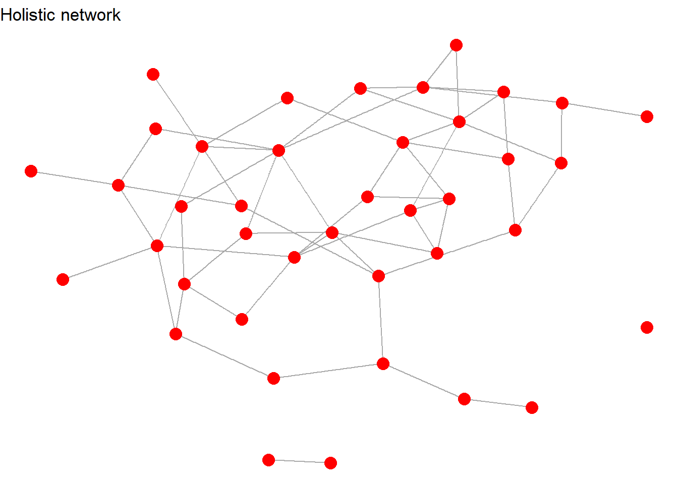
…we obtain multiple smaller networks that revolve around the relationships of a single focal person, ego (which is why these data are referred to as “egocentric”).
n_alters <- 5
ego_id <- 1
alter_ids <- 2:(n_alters + 1)

edges <- data.frame(from = ego_id, to = alter_ids)
alter_pairs <- t(combn(alter_ids, 2))
n_alter_ties <- sample(1:nrow(alter_pairs), 3)
random_alter_edges <- alter_pairs[n_alter_ties, , drop = FALSE]
colnames(random_alter_edges) <- c("from", "to")
edges_all <- rbind(edges, random_alter_edges)

g <- graph_from_data_frame(edges_all, directed = FALSE)
V(g)$label <- c("ego","alter1","alter2","alter3","alter4","alter5")

ggraph(g, layout = "fr") +
  geom_edge_link(color = "gray60") +
  geom_node_point(size = 5, aes(color = label == "ego")) +
  geom_node_text(aes(label = label), vjust = -1, size = 4) +
  scale_color_manual(values = c("TRUE" = "firebrick", "FALSE" = "skyblue"), guide = "none") +
  ggtitle("Egocentric network") +
theme_void() 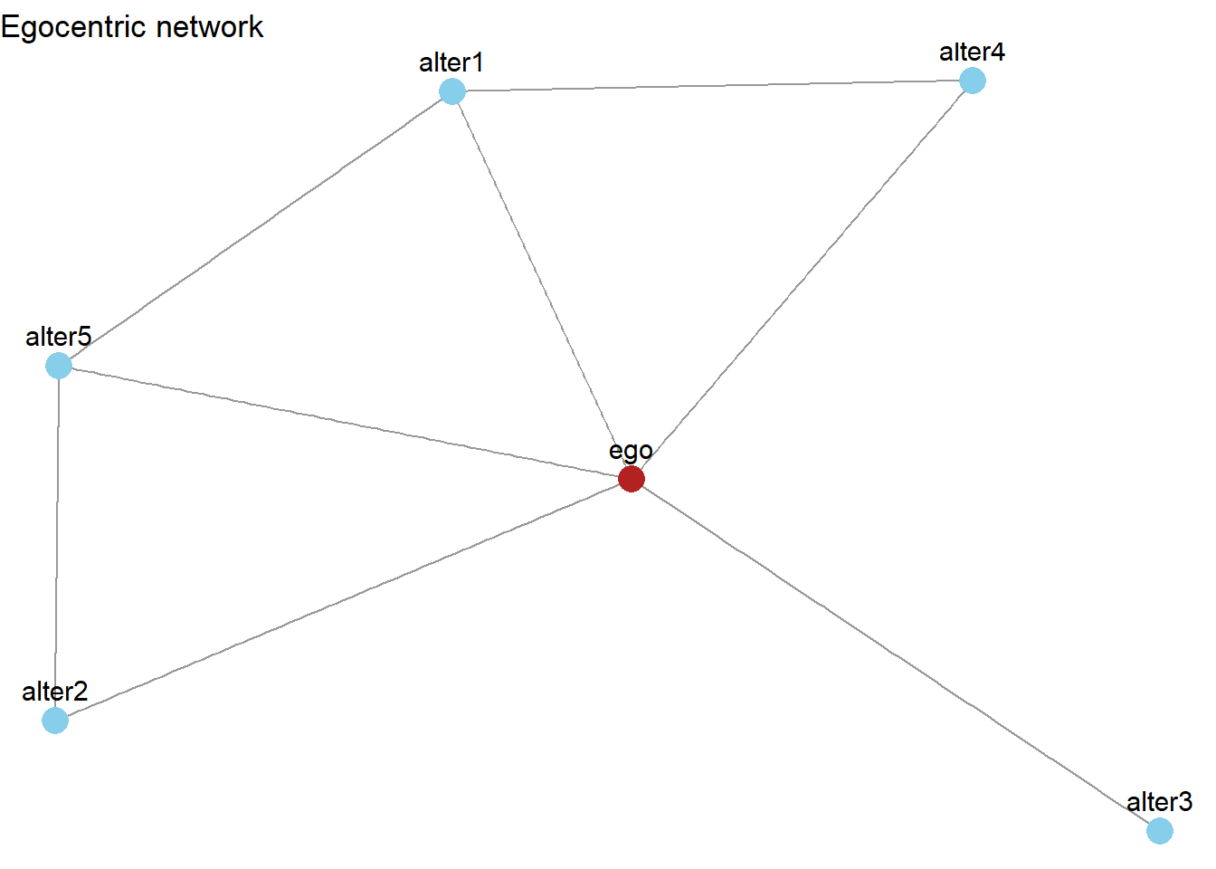
We will demonstrate egocentric network analysis using data from the General Social Survey. Let’s load the data. The “lapply” function sets all of the values in the data matrix to numeric.
setwd("Q:/My Drive/teaching/SOC708/sna/network data/gss04")

# load GSS data
gss <- as.data.frame(as.matrix(read.csv("GSS network data.csv", header=T)))
gss[] <- lapply(gss, as.numeric)
Warning in lapply(gss, as.numeric): NAs introduced by coercionConstructing the files
Ego attributes
Three sets of files are essential for conducting egocentric network analysis. First, we need to gather information about all of the egos – those individuals who were surveyed about their confidants. We therefore subset the gss2 file to include the first eight columns of data, which can then be viewed with the glimpse command.
# save ego attribute data
ego <- gss2[,1:8]
glimpse(ego)
Rows: 288
Columns: 8
$ ego_id <dbl> 3, 5, 10, 12, 16, 30, 35, 36, 46, 54, 57, 59, 61, 62, 63, 65,…
$ AGE <dbl> 52, 34, 26, 58, 48, 73, 47, 58, 55, 49, 47, 55, 49, 40, 40, 5…
$ EDUC <dbl> 14, 17, 14, 12, 11, 16, 17, 16, 16, 12, 16, 16, 16, 16, 20, 2…
$ SEX <dbl> 1, 2, 1, 2, 1, 1, 2, 2, 1, 1, 1, 2, 1, 1, 2, 1, 2, 2, 2, 2, 2…
$ RACE <dbl> 2, 3, 2, 2, 2, 1, 1, 1, 3, 1, 1, 1, 1, 1, 3, 3, 1, 1, 2, 2, 2…
$ PARTYID <dbl> 0, 2, 1, 1, 6, 5, 1, 0, 1, 5, 0, 2, 6, 5, 0, 5, 7, 5, 0, 0, 1…
$ RELIG <dbl> 1, 2, 1, 4, 1, 3, 99, 3, 5, 2, 4, 4, 1, 2, 8, 7, 3, 1, 2, 1, …
$ NUMGIVEN <dbl> 4, 4, 6, 2, 2, 3, 3, 6, 3, 2, 3, 4, 2, 2, 3, 2, 2, 4, 2, 3, 2…For each ego, the data contain a numerical identifier and seven attribute questions. We won’t use all of these variables, but they are available for you to examine if you like.
Alter attributes
Ego was asked to provide information about each of their confidants, which we refer to as alters. So our next step is to construct an alter attribute file. We need the first column of data which includes the ego id, the eight column which is the NUMGIVEN variable, and then a long list of attributes for each alter.
# save alter attribute data
alter <- gss2[,c(1,8,25:114)]
glimpse(alter)
Rows: 288
Columns: 92
$ ego_id <dbl> 3, 5, 10, 12, 16, 30, 35, 36, 46, 54, 57, 59, 61, 62, 63, 65,…
$ NUMGIVEN <dbl> 4, 4, 6, 2, 2, 3, 3, 6, 3, 2, 3, 4, 2, 2, 3, 2, 2, 4, 2, 3, 2…
$ SEX1 <dbl> 2, 2, 2, 2, 1, 1, 1, 2, 1, 1, 1, 1, 2, 1, 1, 1, 1, 2, 1, 2, 2…
$ SEX2 <dbl> 2, 1, 2, 2, 2, 1, 2, 2, 2, 2, 1, 2, 1, 1, 2, 1, 2, 1, 2, 2, 2…
$ SEX3 <dbl> 1, 2, 1, 0, 0, 1, 2, 2, 1, 0, 2, 1, 0, 0, 1, 0, 0, 2, 0, 1, 0…
$ SEX4 <dbl> 1, 2, 2, 0, 0, 0, 0, 1, 0, 0, 0, 1, 0, 0, 0, 0, 0, 1, 0, 0, 0…
$ SEX5 <dbl> 0, 0, 2, 0, 0, 0, 0, 1, 0, 0, 0, 0, 0, 0, 0, 0, 0, 0, 0, 0, 0…
$ RACE1 <dbl> 2, 3, 4, 2, 2, 4, 4, 4, 1, 3, 4, 4, 4, 4, 4, 5, 4, 4, 2, 4, 2…
$ RACE2 <dbl> 2, 3, 2, 4, 2, 4, 4, 4, 1, 3, 1, 4, 4, 4, 4, 5, 4, 4, 2, 3, 2…
$ RACE3 <dbl> 2, 3, 2, 0, 0, 4, 4, 4, 1, 0, 1, 4, 0, 0, 4, 0, 0, 4, 0, 2, 0…
$ RACE4 <dbl> 2, 3, 3, 0, 0, 0, 0, 4, 0, 0, 0, 4, 0, 0, 0, 0, 0, 4, 0, 0, 0…
$ RACE5 <dbl> 0, 0, 3, 0, 0, 0, 0, 4, 0, 0, 0, 0, 0, 0, 0, 0, 0, 0, 0, 0, 0…
$ SPOUSE1 <dbl> 2, 2, 2, 2, 2, 2, 1, 2, 2, 2, 2, 1, 1, 2, 1, 2, 1, 2, 2, 2, 2…
$ SPOUSE2 <dbl> 2, 2, 2, 2, 2, 2, 2, 2, 2, 1, 2, 2, 2, 2, 2, 2, 2, 2, 2, 2, 2…
$ SPOUSE3 <dbl> 2, 2, 2, 0, 0, 2, 2, 2, 2, 0, 2, 2, 0, 0, 2, 0, 0, 2, 0, 2, 0…
$ SPOUSE4 <dbl> 2, 2, 2, 0, 0, 0, 0, 2, 0, 0, 0, 2, 0, 0, 0, 0, 0, 2, 0, 0, 0…
$ SPOUSE5 <dbl> 0, 0, 2, 0, 0, 0, 0, 2, 0, 0, 0, 0, 0, 0, 0, 0, 0, 0, 0, 0, 0…
$ PARENT1 <dbl> 2, 1, 2, 2, 2, 2, 2, 2, 2, 2, 2, 2, 2, 1, 2, 2, 2, 2, 2, 2, 2…
$ PARENT2 <dbl> 2, 2, 2, 2, 2, 2, 2, 2, 2, 2, 2, 2, 2, 2, 2, 2, 2, 2, 2, 2, 1…
$ PARENT3 <dbl> 2, 2, 2, 0, 0, 2, 2, 2, 2, 0, 2, 2, 0, 0, 2, 0, 0, 2, 0, 2, 0…
$ PARENT4 <dbl> 2, 2, 2, 0, 0, 0, 0, 2, 0, 0, 0, 2, 0, 0, 0, 0, 0, 2, 0, 0, 0…
$ PARENT5 <dbl> 0, 0, 2, 0, 0, 0, 0, 2, 0, 0, 0, 0, 0, 0, 0, 0, 0, 0, 0, 0, 0…
$ SIBLING1 <dbl> 2, 2, 2, 2, 2, 1, 2, 2, 1, 1, 2, 2, 2, 2, 2, 2, 2, 2, 2, 2, 2…
$ SIBLING2 <dbl> 2, 2, 2, 2, 2, 2, 2, 2, 2, 2, 2, 2, 2, 2, 1, 2, 2, 2, 2, 2, 2…
$ SIBLING3 <dbl> 2, 2, 2, 0, 0, 2, 2, 2, 2, 0, 2, 1, 0, 0, 2, 0, 0, 2, 0, 2, 0…
$ SIBLING4 <dbl> 1, 2, 2, 0, 0, 0, 0, 2, 0, 0, 0, 1, 0, 0, 0, 0, 0, 1, 0, 0, 0…
$ SIBLING5 <dbl> 0, 0, 2, 0, 0, 0, 0, 2, 0, 0, 0, 0, 0, 0, 0, 0, 0, 0, 0, 0, 0…
$ CHILD1 <dbl> 2, 2, 2, 2, 2, 2, 2, 1, 2, 2, 2, 2, 2, 2, 2, 2, 2, 2, 2, 2, 2…
$ CHILD2 <dbl> 2, 2, 2, 2, 2, 2, 2, 2, 1, 2, 2, 1, 2, 2, 2, 2, 2, 2, 2, 2, 2…
$ CHILD3 <dbl> 2, 2, 2, 0, 0, 2, 2, 2, 2, 0, 2, 2, 0, 0, 2, 0, 0, 2, 0, 2, 0…
$ CHILD4 <dbl> 2, 2, 2, 0, 0, 0, 0, 2, 0, 0, 0, 2, 0, 0, 0, 0, 0, 2, 0, 0, 0…
$ CHILD5 <dbl> 0, 0, 2, 0, 0, 0, 0, 2, 0, 0, 0, 0, 0, 0, 0, 0, 0, 0, 0, 0, 0…
$ OTHFAM1 <dbl> 2, 2, 2, 2, 2, 2, 2, 2, 2, 2, 2, 2, 2, 2, 2, 2, 2, 1, 2, 2, 2…
$ OTHFAM2 <dbl> 2, 2, 2, 2, 2, 2, 1, 2, 2, 2, 2, 2, 1, 1, 2, 1, 2, 1, 2, 2, 2…
$ OTHFAM3 <dbl> 2, 2, 2, 0, 0, 2, 2, 2, 2, 0, 2, 2, 0, 0, 1, 0, 0, 2, 0, 2, 0…
$ OTHFAM4 <dbl> 2, 1, 2, 0, 0, 0, 0, 2, 0, 0, 0, 2, 0, 0, 0, 0, 0, 2, 0, 0, 0…
$ OTHFAM5 <dbl> 0, 0, 2, 0, 0, 0, 0, 2, 0, 0, 0, 0, 0, 0, 0, 0, 0, 0, 0, 0, 0…
$ COWORK1 <dbl> 2, 2, 1, 1, 2, 2, 2, 2, 2, 2, 1, 2, 2, 2, 2, 2, 2, 2, 2, 1, 2…
$ COWORK2 <dbl> 2, 1, 2, 1, 2, 2, 2, 2, 2, 2, 1, 2, 2, 2, 2, 2, 2, 2, 2, 2, 2…
$ COWORK3 <dbl> 2, 1, 1, 0, 0, 2, 2, 2, 2, 0, 1, 2, 0, 0, 2, 0, 0, 2, 0, 2, 0…
$ COWORK4 <dbl> 2, 1, 1, 0, 0, 0, 0, 2, 0, 0, 0, 2, 0, 0, 0, 0, 0, 2, 0, 0, 0…
$ COWORK5 <dbl> 0, 0, 1, 0, 0, 0, 0, 2, 0, 0, 0, 0, 0, 0, 0, 0, 0, 0, 0, 0, 0…
$ MEMGRP1 <dbl> 2, 2, 2, 2, 2, 2, 2, 2, 2, 2, 2, 2, 2, 2, 2, 1, 2, 2, 2, 2, 2…
$ MEMGRP2 <dbl> 2, 2, 2, 2, 2, 2, 2, 2, 2, 2, 2, 2, 2, 1, 2, 2, 2, 2, 2, 2, 2…
$ MEMGRP3 <dbl> 2, 2, 2, 0, 0, 2, 2, 2, 2, 0, 2, 2, 0, 0, 2, 0, 0, 1, 0, 2, 0…
$ MEMGRP4 <dbl> 2, 2, 2, 0, 0, 0, 0, 2, 0, 0, 0, 2, 0, 0, 0, 0, 0, 2, 0, 0, 0…
$ MEMGRP5 <dbl> 0, 0, 2, 0, 0, 0, 0, 2, 0, 0, 0, 0, 0, 0, 0, 0, 0, 0, 0, 0, 0…
$ NEIGHBR1 <dbl> 2, 2, 2, 2, 2, 2, 2, 2, 2, 2, 2, 2, 2, 2, 2, 2, 2, 2, 2, 2, 2…
$ NEIGHBR2 <dbl> 2, 2, 2, 2, 2, 2, 2, 2, 2, 2, 2, 2, 2, 1, 2, 2, 2, 2, 2, 2, 2…
$ NEIGHBR3 <dbl> 2, 2, 2, 0, 0, 2, 2, 2, 2, 0, 2, 2, 0, 0, 2, 0, 0, 2, 0, 2, 0…
$ NEIGHBR4 <dbl> 2, 2, 2, 0, 0, 0, 0, 2, 0, 0, 0, 2, 0, 0, 0, 0, 0, 2, 0, 0, 0…
$ NEIGHBR5 <dbl> 0, 0, 2, 0, 0, 0, 0, 2, 0, 0, 0, 0, 0, 0, 0, 0, 0, 0, 0, 0, 0…
$ FRIEND1 <dbl> 1, 2, 2, 2, 2, 2, 2, 2, 1, 2, 1, 2, 2, 2, 2, 2, 2, 2, 1, 1, 1…
$ FRIEND2 <dbl> 1, 1, 1, 2, 2, 1, 2, 1, 1, 2, 1, 2, 2, 2, 2, 2, 1, 2, 2, 1, 2…
$ FRIEND3 <dbl> 1, 1, 2, 0, 0, 1, 2, 1, 1, 0, 1, 2, 0, 0, 2, 0, 0, 2, 0, 1, 0…
$ FRIEND4 <dbl> 2, 2, 2, 0, 0, 0, 0, 1, 0, 0, 0, 2, 0, 0, 0, 0, 0, 2, 0, 0, 0…
$ FRIEND5 <dbl> 0, 0, 2, 0, 0, 0, 0, 1, 0, 0, 0, 0, 0, 0, 0, 0, 0, 0, 0, 0, 0…
$ ADVISOR1 <dbl> 2, 2, 2, 2, 1, 2, 2, 2, 1, 2, 2, 2, 2, 2, 2, 2, 2, 2, 2, 2, 2…
$ ADVISOR2 <dbl> 2, 2, 2, 2, 1, 2, 2, 2, 1, 2, 2, 2, 2, 2, 2, 2, 2, 2, 2, 2, 2…
$ ADVISOR3 <dbl> 2, 2, 2, 0, 0, 2, 2, 2, 1, 0, 2, 2, 0, 0, 2, 0, 0, 2, 0, 2, 0…
$ ADVISOR4 <dbl> 2, 2, 2, 0, 0, 0, 0, 2, 0, 0, 0, 2, 0, 0, 0, 0, 0, 2, 0, 0, 0…
$ ADVISOR5 <dbl> 0, 0, 2, 0, 0, 0, 0, 2, 0, 0, 0, 0, 0, 0, 0, 0, 0, 0, 0, 0, 0…
$ OTHER1 <dbl> 2, 2, 2, 2, 2, 2, 2, 2, 2, 1, 2, 2, 2, 1, 2, 2, 2, 2, 2, 2, 2…
$ OTHER2 <dbl> 2, 2, 2, 2, 2, 2, 2, 2, 2, 2, 2, 2, 2, 2, 2, 2, 2, 2, 1, 2, 2…
$ OTHER3 <dbl> 2, 2, 2, 0, 0, 2, 1, 2, 2, 0, 2, 2, 0, 0, 2, 0, 0, 2, 0, 2, 0…
$ OTHER4 <dbl> 2, 2, 2, 0, 0, 0, 0, 2, 0, 0, 0, 2, 0, 0, 0, 0, 0, 2, 0, 0, 0…
$ OTHER5 <dbl> 0, 0, 2, 0, 0, 0, 0, 2, 0, 0, 0, 0, 0, 0, 0, 0, 0, 0, 0, 0, 0…
$ TALKTO1 <dbl> 4, 1, 1, 2, 2, 4, 1, 1, 2, 1, 1, 1, 1, 2, 1, 1, 1, 3, 3, 1, 1…
$ TALKTO2 <dbl> 1, 1, 1, 2, 2, 3, 1, 2, 1, 1, 1, 2, 4, 2, 1, 2, 1, 2, 3, 1, 1…
$ TALKTO3 <dbl> 2, 1, 1, 0, 0, 1, 2, 3, 2, 0, 1, 4, 0, 0, 3, 0, 0, 1, 0, 1, 0…
$ TALKTO4 <dbl> 2, 1, 3, 0, 0, 0, 0, 3, 0, 0, 0, 3, 0, 0, 0, 0, 0, 3, 0, 0, 0…
$ TALKTO5 <dbl> 0, 0, 1, 0, 0, 0, 0, 2, 0, 0, 0, 0, 0, 0, 0, 0, 0, 0, 0, 0, 0…
$ KNOWN1 <dbl> 0, 0, 0, 0, 0, 0, 0, 0, 0, 0, 0, 0, 0, 0, 0, 0, 0, 0, 0, 0, 0…
$ KNOWN2 <dbl> 0, 0, 0, 0, 0, 0, 0, 0, 0, 0, 0, 0, 0, 0, 0, 0, 0, 0, 0, 0, 0…
$ KNOWN3 <dbl> 0, 0, 0, 0, 0, 0, 0, 0, 0, 0, 0, 0, 0, 0, 0, 0, 0, 0, 0, 0, 0…
$ KNOWN4 <dbl> 0, 0, 0, 0, 0, 0, 0, 0, 0, 0, 0, 0, 0, 0, 0, 0, 0, 0, 0, 0, 0…
$ KNOWN5 <dbl> 0, 0, 0, 0, 0, 0, 0, 0, 0, 0, 0, 0, 0, 0, 0, 0, 0, 0, 0, 0, 0…
$ EDUC1 <dbl> 6, 7, 3, 3, 8, 7, 7, 6, 3, 3, 7, 7, 6, 0, 7, 7, 7, 3, 6, 5, 4…
$ EDUC2 <dbl> 3, 3, 3, 6, 8, 6, 6, 6, 7, 3, 7, 6, 7, 6, 7, 7, 7, 7, 7, 6, 6…
$ EDUC3 <dbl> 7, 7, 3, -1, -1, 6, 7, 7, 6, -1, 7, 6, -1, -1, 7, -1, -1, 4, …
$ EDUC4 <dbl> 6, 7, 4, -1, -1, -1, -1, 7, -1, -1, -1, 6, -1, -1, -1, -1, -1…
$ EDUC5 <dbl> -1, -1, 4, -1, -1, -1, -1, 7, -1, -1, -1, -1, -1, -1, -1, -1,…
$ AGE1 <dbl> 56, 63, 25, 57, 50, 69, 47, 25, 50, 47, 55, 54, 48, 77, 43, 9…
$ AGE2 <dbl> 40, 36, 25, 52, 98, 62, 79, 57, 24, 34, 50, 27, 72, 64, 40, 4…
$ AGE3 <dbl> 58, 34, 39, -1, -1, 60, 55, 57, 52, -1, 35, 59, -1, -1, 41, -…
$ AGE4 <dbl> 59, 36, 33, -1, -1, -1, -1, 59, -1, -1, -1, 58, -1, -1, -1, -…
$ AGE5 <dbl> -1, -1, 30, -1, -1, -1, -1, 57, -1, -1, -1, -1, -1, -1, -1, -…
$ RELIG1 <dbl> 1, 2, 5, 2, 8, 3, 9, 3, 4, 2, 1, 4, 1, 2, 5, 8, 3, 2, 4, 1, 1…
$ RELIG2 <dbl> 1, 2, 5, 3, 8, 3, 9, 3, 4, 2, 5, 2, 1, 2, 5, 5, 3, 1, 2, 1, 1…
$ RELIG3 <dbl> 1, 2, 2, 0, 0, 3, 9, 3, 5, 0, 8, 2, 0, 0, 4, 0, 0, 1, 0, 1, 0…
$ RELIG4 <dbl> 1, 2, 2, 0, 0, 0, 0, 3, 0, 0, 0, 2, 0, 0, 0, 0, 0, 1, 0, 0, 0…
$ RELIG5 <dbl> 0, 0, 2, 0, 0, 0, 0, 3, 0, 0, 0, 0, 0, 0, 0, 0, 0, 0, 0, 0, 0…The alter attributes include a number at the end of the variable name to indicate which which alter is being referenced. Note that these numbers range from 1 to 5. So if an ego said that they confide in 6 or more alters, the GSS collected information on only the first five alters. Consequently, the maximum number of ego network alters in our analysis will be five.
At present, the data are organized by unique egos. But what we really want is for each line to represent a unique alter. In data management speak, the current file is in “wide” format (with the data extending out to the right as variables for separate alters) and needs to be transformed to “long” format (with the data for each alter extending down for each alter). If an ego has three alters, then there should be three rows in the data, one for each alter.
To accomplish this, use the pivot_longer command. The code below reshapes the existing data from wide to long format, extending down information for each alter (so all columns except for ego_id and NUMGIVEN, which we want to repeat for each ego). The names_ functions tell R how to rename the variables (SPOUSE1 should become SPOUSE) and create an alter id variable (and formatting that variable is numeric).
# reshape alter attributes
alterlong <- alter |>
  pivot_longer(
    cols = -c(ego_id,NUMGIVEN),
    names_to = c(".value", "alter_id"),  # Split names into "base" and "set" parts
    names_pattern = "(\\D+)(\\d+)"  # Separate variable base and set number
  )

# change alter_id to numeric variable
alterlong$alter_id <- as.numeric(alterlong$alter_id)
Let’s inspect this file before making further adjustments.
glimpse(alterlong)Rows: 1,440
Columns: 21
$ ego_id <dbl> 3, 3, 3, 3, 3, 5, 5, 5, 5, 5, 10, 10, 10, 10, 10, 12, 12, 12,…
$ NUMGIVEN <dbl> 4, 4, 4, 4, 4, 4, 4, 4, 4, 4, 6, 6, 6, 6, 6, 2, 2, 2, 2, 2, 2…
$ alter_id <dbl> 1, 2, 3, 4, 5, 1, 2, 3, 4, 5, 1, 2, 3, 4, 5, 1, 2, 3, 4, 5, 1…
$ SEX <dbl> 2, 2, 1, 1, 0, 2, 1, 2, 2, 0, 2, 2, 1, 2, 2, 2, 2, 0, 0, 0, 1…
$ RACE <dbl> 2, 2, 2, 2, 0, 3, 3, 3, 3, 0, 4, 2, 2, 3, 3, 2, 4, 0, 0, 0, 2…
$ SPOUSE <dbl> 2, 2, 2, 2, 0, 2, 2, 2, 2, 0, 2, 2, 2, 2, 2, 2, 2, 0, 0, 0, 2…
$ PARENT <dbl> 2, 2, 2, 2, 0, 1, 2, 2, 2, 0, 2, 2, 2, 2, 2, 2, 2, 0, 0, 0, 2…
$ SIBLING <dbl> 2, 2, 2, 1, 0, 2, 2, 2, 2, 0, 2, 2, 2, 2, 2, 2, 2, 0, 0, 0, 2…
$ CHILD <dbl> 2, 2, 2, 2, 0, 2, 2, 2, 2, 0, 2, 2, 2, 2, 2, 2, 2, 0, 0, 0, 2…
$ OTHFAM <dbl> 2, 2, 2, 2, 0, 2, 2, 2, 1, 0, 2, 2, 2, 2, 2, 2, 2, 0, 0, 0, 2…
$ COWORK <dbl> 2, 2, 2, 2, 0, 2, 1, 1, 1, 0, 1, 2, 1, 1, 1, 1, 1, 0, 0, 0, 2…
$ MEMGRP <dbl> 2, 2, 2, 2, 0, 2, 2, 2, 2, 0, 2, 2, 2, 2, 2, 2, 2, 0, 0, 0, 2…
$ NEIGHBR <dbl> 2, 2, 2, 2, 0, 2, 2, 2, 2, 0, 2, 2, 2, 2, 2, 2, 2, 0, 0, 0, 2…
$ FRIEND <dbl> 1, 1, 1, 2, 0, 2, 1, 1, 2, 0, 2, 1, 2, 2, 2, 2, 2, 0, 0, 0, 2…
$ ADVISOR <dbl> 2, 2, 2, 2, 0, 2, 2, 2, 2, 0, 2, 2, 2, 2, 2, 2, 2, 0, 0, 0, 1…
$ OTHER <dbl> 2, 2, 2, 2, 0, 2, 2, 2, 2, 0, 2, 2, 2, 2, 2, 2, 2, 0, 0, 0, 2…
$ TALKTO <dbl> 4, 1, 2, 2, 0, 1, 1, 1, 1, 0, 1, 1, 1, 3, 1, 2, 2, 0, 0, 0, 2…
$ KNOWN <dbl> 0, 0, 0, 0, 0, 0, 0, 0, 0, 0, 0, 0, 0, 0, 0, 0, 0, 0, 0, 0, 0…
$ EDUC <dbl> 6, 3, 7, 6, -1, 7, 3, 7, 7, -1, 3, 3, 3, 4, 4, 3, 6, -1, -1, …
$ AGE <dbl> 56, 40, 58, 59, -1, 63, 36, 34, 36, -1, 25, 25, 39, 33, 30, 5…
$ RELIG <dbl> 1, 1, 1, 1, 0, 2, 2, 2, 2, 0, 5, 5, 2, 2, 2, 2, 3, 0, 0, 0, 8…This new alterlong file has exactly five times the number of observations as the original alter file (288*5 = 1440). That’s because each ego now has five lines, given the potential for having up to five different alters. Alterlong also has much fewer variables, because each of the attributes that used to have five different variables (PARENT1-5) now has only a single variable (PARENT).
This dataset contains multiple rows with missing information. For example, the first five entries are for ego_id = 3. The NUMGIVEN value of 4 indicates that this person reported 4 alters. The first 4 entries contain valid alter information, but the 5th entry contains 0s or -1s, which are invalid. Therefore, we need to delete all of the rows for alters that do not exist. Then we can remove the NUMGIVEN variable because it is no longer needed.
# keep only rows where ALTERID <= NUMGIVEN
# these rows refer to alters that do not exist in the data
# then remove NUMGIVEN
alterlong <- alterlong |>
  filter(alter_id <= NUMGIVEN) |>
  select(-NUMGIVEN)
The next step is to adjust the alter_id variables. At present, those ids (1-5) repeat across the dataset, so they are not unique. A better approach is to create unique identifiers that provide information not only about the number designation for the alter, but also the number of the ego to whom they are attached. The code below does this by multiplying the ego_id by 10 and then adding the alter_id.
# distinct ID values
alterlong$alter_id <- alterlong$ego_id*10 + alterlong$alter_id
glimpse(alterlong[,1:2])
Rows: 955
Columns: 2
$ ego_id <dbl> 3, 3, 3, 3, 5, 5, 5, 5, 10, 10, 10, 10, 10, 12, 12, 16, 16, 3…
$ alter_id <dbl> 31, 32, 33, 34, 51, 52, 53, 54, 101, 102, 103, 104, 105, 121,…Now we can see that ego #10’s 4th alter has an alter_id of 104. This will be very helpful when we visualize these networks later.
Alter edgelist
An edgelist is also needed. For this file, we’ll save the first column (ego_id) and columns 15-24.
# save edge data
edges <- gss2[,c(1,15:24)]
glimpse(edges)
Rows: 288
Columns: 11
$ ego_id <dbl> 3, 5, 10, 12, 16, 30, 35, 36, 46, 54, 57, 59, 61, 62, 63, 65, …
$ CLOSE12 <dbl> 2, 1, 3, 3, 3, 2, 2, 2, 2, 3, 1, 1, 1, 2, 2, 3, 2, 1, 2, 3, 1,…
$ CLOSE13 <dbl> 1, 3, 1, 0, 0, 2, 2, 2, 2, 0, 1, 2, 0, 0, 2, 0, 0, 1, 0, 2, 0,…
$ CLOSE14 <dbl> 3, 1, 2, 0, 0, 0, 0, 2, 0, 0, 0, 2, 0, 0, 0, 0, 0, 1, 0, 0, 0,…
$ CLOSE15 <dbl> 0, 0, 2, 0, 0, 0, 0, 1, 0, 0, 0, 0, 0, 0, 0, 0, 0, 0, 0, 0, 0,…
$ CLOSE23 <dbl> 1, 1, 2, 0, 0, 2, 3, 2, 2, 0, 2, 2, 0, 0, 1, 0, 0, 1, 0, 2, 0,…
$ CLOSE24 <dbl> 1, 1, 2, 0, 0, 0, 0, 2, 0, 0, 0, 2, 0, 0, 0, 0, 0, 1, 0, 0, 0,…
$ CLOSE25 <dbl> 0, 0, 2, 0, 0, 0, 0, 2, 0, 0, 0, 0, 0, 0, 0, 0, 0, 0, 0, 0, 0,…
$ CLOSE34 <dbl> 2, 1, 1, 0, 0, 0, 0, 1, 0, 0, 0, 2, 0, 0, 0, 0, 0, 1, 0, 0, 0,…
$ CLOSE35 <dbl> 0, 0, 1, 0, 0, 0, 0, 2, 0, 0, 0, 0, 0, 0, 0, 0, 0, 0, 0, 0, 0,…
$ CLOSE45 <dbl> 0, 0, 1, 0, 0, 0, 0, 2, 0, 0, 0, 0, 0, 0, 0, 0, 0, 0, 0, 0, 0,…These variables measure how close ego thinks that the two alters are to one another. We will examine the specific values later. For now, just note that the numbers indicate which alters are being referenced. For example, CLOSE25 refers to the perceive closeness between alter 2 and alter 5.
To create the edgelist, we need to pivot_long (like before) so that each line represents a unique relationship between alters.
# reshape edges long
edgeslong <- edges  |>
  pivot_longer(
    cols = -ego_id,
    names_to = "tie",     # Name for the column representing each tie variable
    values_to = "weight"  # Name for the tie strength values
  ) |>
  mutate(
    from = as.integer(sub("CLOSE(\\d)(\\d)", "\\1", tie)),  # Extract first alter from tie variable
    to = as.integer(sub("CLOSE(\\d)(\\d)", "\\2", tie))   # Extract second alter from tie variable
  ) |>
  select(ego_id, from, to, weight)
glimpse(edgeslong)
Rows: 2,880
Columns: 4
$ ego_id <dbl> 3, 3, 3, 3, 3, 3, 3, 3, 3, 3, 5, 5, 5, 5, 5, 5, 5, 5, 5, 5, 10,…
$ from <int> 1, 1, 1, 1, 2, 2, 2, 3, 3, 4, 1, 1, 1, 1, 2, 2, 2, 3, 3, 4, 1, …
$ to <int> 2, 3, 4, 5, 3, 4, 5, 4, 5, 5, 2, 3, 4, 5, 3, 4, 5, 4, 5, 5, 2, …
$ weight <dbl> 2, 1, 3, 0, 1, 1, 0, 2, 0, 0, 1, 3, 1, 0, 1, 1, 0, 1, 0, 0, 3, …In addition to the ego_id we have “from” and “to” variables which contain the numbers of the alters that are connected. The direction of the tie does not matter as these relationships are assumed to be symmetric.
The weight variable tells us about the strength of the tie between each alter. Oddly, the GSS coded greater closeness between alters with descending values. It makes more sense to recode closer friends (“especially close”) with higher values, which we do below. Also, “total strangers” indicates that there is no relationship, so those lines are removed from the dataset.
# 1 ESPECIALLY CLOSE; 2 KNOW EACH OTHER; 3  TOTAL STRANGERS
# recode 1->2, 2->1, 3->0, then remove zeros
edgeslong <- edgeslong |>
  mutate(weight = recode(weight, `1`=2, `2`=1, `3`=0)) |>
  filter(weight > 0)
Now we need to adjust the id values for the alters so they match with the alter attribute file.
# consistent IDs that will link with the alter attribute files
edgeslong$from <- edgeslong$ego_id*10 + edgeslong$from
edgeslong$to <- edgeslong$ego_id*10 + edgeslong$to
glimpse(edgeslong)
Rows: 1,030
Columns: 4
$ ego_id <dbl> 3, 3, 3, 3, 3, 5, 5, 5, 5, 5, 10, 10, 10, 10, 10, 10, 10, 10, 1…
$ from <dbl> 31, 31, 32, 32, 33, 51, 51, 52, 52, 53, 101, 101, 101, 102, 102…
$ to <dbl> 32, 33, 33, 34, 34, 52, 54, 53, 54, 54, 103, 104, 105, 103, 104…
$ weight <dbl> 1, 2, 2, 2, 1, 2, 2, 2, 2, 2, 2, 1, 1, 1, 1, 1, 2, 2, 2, 1, 1, …egor
Now that the files are prepped, they can be combined into an “egor” object. egor is a package designed for conducting egocentric network analysis. The code below loads the egor package and combines the various files we just created into an egor object.
# Create an egor object
library(egor)
egor.obj <- egor(egos = ego,
                 alters = alterlong,
                 aaties = edgeslong,
                 ID.vars = list(ego = "ego_id",
                                alter = "alter_id",
                                source = "from",
                                target = "to"))
The next step is to convert the egor object into an igraph object. Then we can examine the object.
# transform into an igraph object
gr.list <- as_igraph(egor.obj)
head(gr.list)
$`3`
IGRAPH 3e7e826 UNW- 4 5 --
+ attr: .egoID (g/n), name (v/c), SEX (v/n), RACE (v/n), SPOUSE (v/n),
| PARENT (v/n), SIBLING (v/n), CHILD (v/n), OTHFAM (v/n), COWORK (v/n),
| MEMGRP (v/n), NEIGHBR (v/n), FRIEND (v/n), ADVISOR (v/n), OTHER
| (v/n), TALKTO (v/n), KNOWN (v/n), EDUC (v/n), AGE (v/n), RELIG (v/n),
| weight (e/n)
+ edges from 3e7e826 (vertex names):
[1] 31--32 31--33 32--33 32--34 33--34
$`5`
IGRAPH 3e7eee4 UNW- 4 5 --
+ attr: .egoID (g/n), name (v/c), SEX (v/n), RACE (v/n), SPOUSE (v/n),
| PARENT (v/n), SIBLING (v/n), CHILD (v/n), OTHFAM (v/n), COWORK (v/n),
| MEMGRP (v/n), NEIGHBR (v/n), FRIEND (v/n), ADVISOR (v/n), OTHER
| (v/n), TALKTO (v/n), KNOWN (v/n), EDUC (v/n), AGE (v/n), RELIG (v/n),
| weight (e/n)
+ edges from 3e7eee4 (vertex names):
[1] 51--52 51--54 52--53 52--54 53--54
$`10`
IGRAPH 3e7f81c UNW- 5 9 --
+ attr: .egoID (g/n), name (v/c), SEX (v/n), RACE (v/n), SPOUSE (v/n),
| PARENT (v/n), SIBLING (v/n), CHILD (v/n), OTHFAM (v/n), COWORK (v/n),
| MEMGRP (v/n), NEIGHBR (v/n), FRIEND (v/n), ADVISOR (v/n), OTHER
| (v/n), TALKTO (v/n), KNOWN (v/n), EDUC (v/n), AGE (v/n), RELIG (v/n),
| weight (e/n)
+ edges from 3e7f81c (vertex names):
[1] 101--103 101--104 101--105 102--103 102--104 102--105 103--104 103--105
[9] 104--105
$`12`
IGRAPH 3e803c3 UNW- 2 0 --
+ attr: .egoID (g/n), name (v/c), SEX (v/n), RACE (v/n), SPOUSE (v/n),
| PARENT (v/n), SIBLING (v/n), CHILD (v/n), OTHFAM (v/n), COWORK (v/n),
| MEMGRP (v/n), NEIGHBR (v/n), FRIEND (v/n), ADVISOR (v/n), OTHER
| (v/n), TALKTO (v/n), KNOWN (v/n), EDUC (v/n), AGE (v/n), RELIG (v/n),
| weight (e/n)
+ edges from 3e803c3 (vertex names):
$`16`
IGRAPH 3e80af8 UNW- 2 0 --
+ attr: .egoID (g/n), name (v/c), SEX (v/n), RACE (v/n), SPOUSE (v/n),
| PARENT (v/n), SIBLING (v/n), CHILD (v/n), OTHFAM (v/n), COWORK (v/n),
| MEMGRP (v/n), NEIGHBR (v/n), FRIEND (v/n), ADVISOR (v/n), OTHER
| (v/n), TALKTO (v/n), KNOWN (v/n), EDUC (v/n), AGE (v/n), RELIG (v/n),
| weight (e/n)
+ edges from 3e80af8 (vertex names):
$`30`
IGRAPH 3e810ff UNW- 3 3 --
+ attr: .egoID (g/n), name (v/c), SEX (v/n), RACE (v/n), SPOUSE (v/n),
| PARENT (v/n), SIBLING (v/n), CHILD (v/n), OTHFAM (v/n), COWORK (v/n),
| MEMGRP (v/n), NEIGHBR (v/n), FRIEND (v/n), ADVISOR (v/n), OTHER
| (v/n), TALKTO (v/n), KNOWN (v/n), EDUC (v/n), AGE (v/n), RELIG (v/n),
| weight (e/n)
+ edges from 3e810ff (vertex names):
[1] 301--302 301--303 302--303This new object looks a bit different from the igraph objects we’ve looked at in the past. Embedded in this object is not one single network, but multiple networks, with each element’s name corresponding to the ego ID.
names(gr.list) [1] "3" "5" "10" "12" "16" "30" "35" "36" "46" "54" "57" "59"
[13] "61" "62" "63" "65" "66" "70" "71" "72" "74" "75" "80" "83"
[25] "84" "90" "92" "93" "94" "95" "103" "106" "112" "116" "117" "125"
[37] "129" "131" "133" "135" "136" "139" "140" "144" "152" "155" "160" "166"
[49] "171" "177" "181" "184" "185" "193" "198" "199" "202" "218" "220" "223"
[61] "229" "233" "235" "237" "238" "239" "250" "252" "253" "255" "258" "259"
[73] "261" "262" "266" "268" "269" "270" "271" "276" "278" "280" "281" "284"
[85] "285" "289" "294" "296" "299" "300" "301" "302" "305" "314" "316" "317"
[97] "320" "322" "323" "326" "330" "331" "336" "337" "340" "345" "350" "353"
[109] "355" "356" "358" "359" "360" "361" "363" "365" "366" "370" "372" "373"
[121] "375" "377" "378" "381" "382" "391" "392" "393" "394" "396" "397" "401"
[133] "402" "403" "407" "410" "412" "413" "414" "420" "424" "431" "433" "441"
[145] "448" "449" "457" "460" "462" "465" "471" "472" "475" "476" "485" "487"
[157] "489" "490" "501" "511" "522" "523" "530" "539" "542" "544" "554" "555"
[169] "559" "560" "561" "563" "567" "568" "569" "572" "582" "587" "589" "590"
[181] "595" "598" "603" "617" "618" "630" "635" "636" "642" "669" "672" "676"
[193] "683" "686" "688" "690" "691" "694" "699" "708" "710" "713" "714" "715"
[205] "717" "726" "729" "733" "734" "742" "744" "746" "748" "756" "758" "759"
[217] "763" "764" "768" "769" "770" "773" "780" "781" "784" "788" "789" "790"
[229] "794" "797" "801" "803" "805" "808" "811" "813" "816" "821" "828" "829"
[241] "835" "836" "841" "843" "844" "846" "847" "848" "855" "864" "873" "876"
[253] "877" "878" "885" "887" "893" "899" "902" "905" "906" "912" "915" "919"
[265] "920" "921" "927" "936" "939" "941" "942" "944" "945" "950" "952" "957"
[277] "958" "967" "975" "976" "978" "983" "988" "994" "995" "997" "998" "999"Note that this set of networks only includes the alter-alter ties. We may want to generate another set of networks in which ego is also included. This can be done using the include.ego option.
gr.list.ego <- as_igraph(egor.obj, include.ego = TRUE)Examining the egonet objects
Now let’s take a closer look at the first egonet object. To do this, we can subset the gr.list with a double bracket. Then let’s look at the vertex sequence.
(gr <- gr.list[["3"]])IGRAPH 3e7e826 UNW- 4 5 --
+ attr: .egoID (g/n), name (v/c), SEX (v/n), RACE (v/n), SPOUSE (v/n),
| PARENT (v/n), SIBLING (v/n), CHILD (v/n), OTHFAM (v/n), COWORK (v/n),
| MEMGRP (v/n), NEIGHBR (v/n), FRIEND (v/n), ADVISOR (v/n), OTHER
| (v/n), TALKTO (v/n), KNOWN (v/n), EDUC (v/n), AGE (v/n), RELIG (v/n),
| weight (e/n)
+ edges from 3e7e826 (vertex names):
[1] 31--32 31--33 32--33 32--34 33--34V(gr)+ 4/4 vertices, named, from 3e7e826:
[1] 31 32 33 34What if we examined the vertex sequence with ego included? Note the name of the last node.
(gr.ego <- gr.list.ego[["3"]])IGRAPH 3f89904 UNW- 5 9 --
+ attr: .egoID (g/n), name (v/c), SEX (v/n), RACE (v/n), SPOUSE (v/n),
| PARENT (v/n), SIBLING (v/n), CHILD (v/n), OTHFAM (v/n), COWORK (v/n),
| MEMGRP (v/n), NEIGHBR (v/n), FRIEND (v/n), ADVISOR (v/n), OTHER
| (v/n), TALKTO (v/n), KNOWN (v/n), EDUC (v/n), AGE (v/n), RELIG (v/n),
| weight (e/n)
+ edges from 3f89904 (vertex names):
[1] 31--32 31--33 32--33 32--34 33--34 31--ego 32--ego 33--ego 34--egoV(gr.ego)+ 5/5 vertices, named, from 3f89904:
[1] 31 32 33 34 egoNow let’s plot out the two versions of this ego network: one without ego and one with ego included.
par(mar = c(0,0,2,0), mfrow = c(1,2))
plot(gr, vertex.label = NA, main = "No ego")
plot(gr.ego, vertex.label = NA, main = "With ego")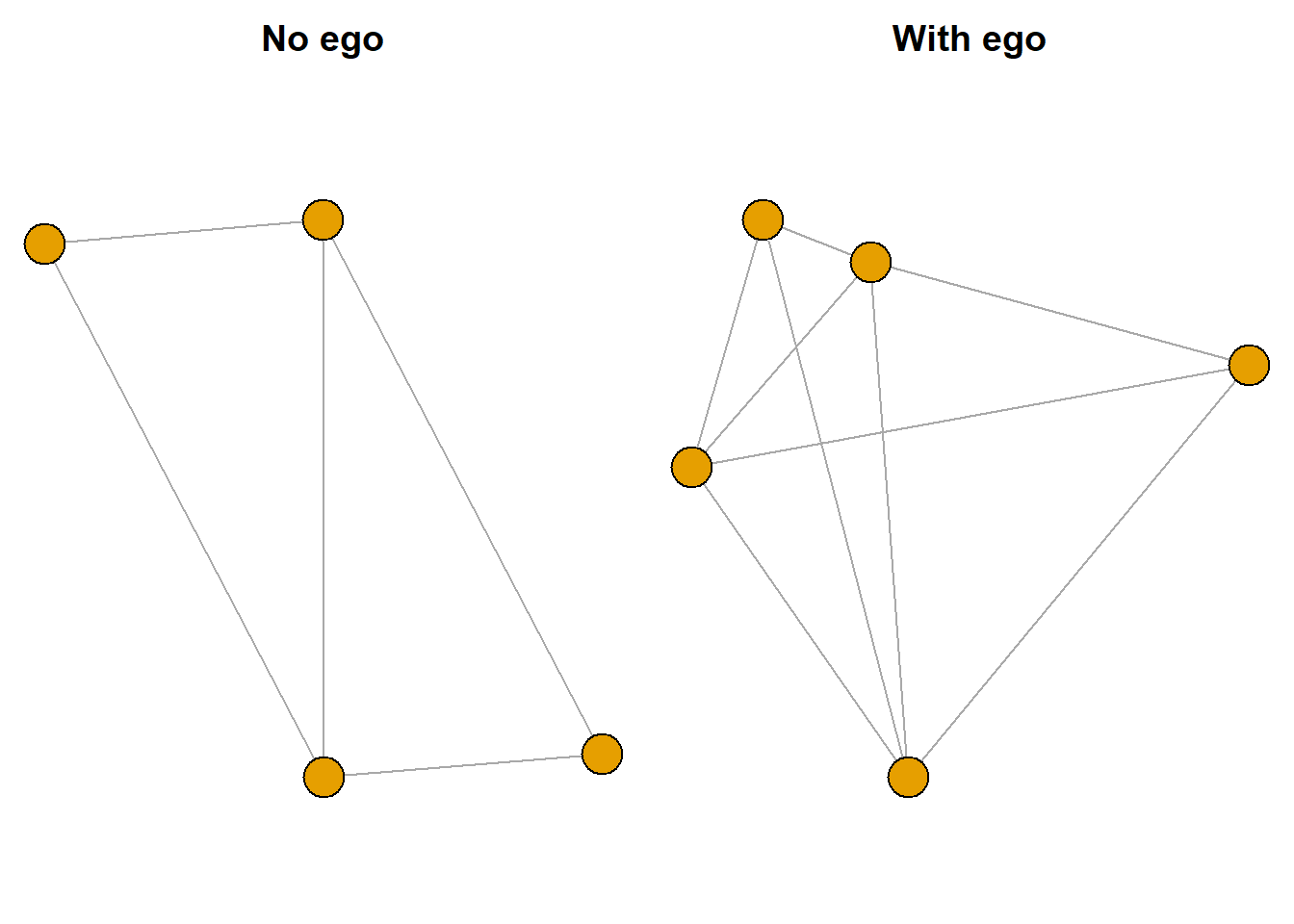
In the “With ego” graph, can you pick out which node is ego? Remember that ego will always be connected to all nodes in the graph.
The next step is to add ego ID as a graph attribute in each list element. We will do this for the alter only object and the ego included object. This will be useful when graphing the different ego networks.
# List of graphs without ego
for (i in seq_along(gr.list)) {
  gr.list[[i]]$ego_id <- names(gr.list)[[i]]
}

# List of graphs with ego
for (i in seq_along(gr.list.ego)) {
  gr.list.ego[[i]]$ego_id <- names(gr.list.ego)[[i]]
}

gr.list[["10"]]$ego_id
[1] "10"Now that the ego network data have been properly formatted, we can save the objects as an R readable .rda file. We will load these objects and examine them in the next tutorial.
# Save data to file
save(ego, alterlong, gr.list, gr.list.ego, file="gss_ego.rda")
References
This tutorial was built on insights and code from Raffaele Vacca. Please see his textbook (https://raffaelevacca.github.io/egocentric-r-book/) for a more detailed discussion of ego networks.
If you are interested in some of the substantive issues associated with the GSS “important matters” network data, check out the following resources.
Bearman, Peter, and Paolo Parigi. 2004. “Cloning Headless Frogs and Other Important Matters: Conversation Topics and Network Structure.” Social Forces 83(2):535–57.
Fischer, Claude S. 2009. “The 2004 GSS Finding of Shrunken Social Networks: An Artifact?” American Sociological Review 74(4):657–69.
McPherson, Miller, Lynn Smith-Lovin, and Matthew E. Brashears. 2006. “Social Isolation in America: Changes in Core Discussion Networks over Two Decades.” American Sociological Review 71(3):353–75.
Small, Mario Luis. 2017. Someone to Talk To. Oxford University Press.
Smith, Jeffrey A., Miller McPherson, and Lynn Smith-Lovin. 2014. “Social Distance in the United States: Sex, Race, Religion, Age, and Education Homophily among Confidants, 1985 to 2004.” American Sociological Review 79(3):432–56.